Life-threatening, extreme heat arrived early in India, Pakistan, and other parts of south Asia this year, exposing more than 1 billion people—more than 10% of the world’s population—to increased health risks. If global average temperatures rise 1.5 degrees Celsius (2.7° Fahrenheit) above pre-industrial levels, extreme heat and humidity are expected to impact areas currently home to populations of this size annually, with heat stress affecting more than 12 times the number of people compared to a world without climate change.

As we face the punishing impacts of global climate change it can be easy to wonder, do efforts to reduce emissions by individual countries, states or cities really make a difference? Research by the Climate Impact Lab, which measures the economic and social costs of climate change, can help answer this question. The Lab developed the first global, empirically-based model of the impact of climate-driven changes in temperatures on human mortality rates. A new tool built by the Lab uses this model to quantify how many lives could be saved around the world from reduced emissions within the U.S.—whether at the town, city, state, or national level. The tool also measures how much money the global economy would save through avoided costs of adapting to increased mortality risk. Using this new Lives Saved Calculator, the marginal benefits of each single ton of carbon emissions avoided become evident. For instance, 10 states have set goals of 100% clean electricity by 2050 or earlier. Achieving those targets would save 221,000 lives and avoid $101 billion in adaptation costs through the end of the century. Achieving net-zero emissions economy-wide in these states would save an additional 993,000 lives.

Introducing the Lives Saved Calculator

Much of the Climate Impact Lab’s work focuses on quantifying the long-run impact of each additional ton of carbon dioxide (CO₂) released into the atmosphere on a range of economic and social outcomes, from farm yields to labor productivity to energy costs. New research, forthcoming in the Quarterly Journal of Economics, quantifies the impact of an additional ton of CO₂ on death rates around the world and the costly adaptations that people make to protect themselves from heat. This same model can be applied to quantify the benefit of avoiding even 1 ton of carbon dioxide (CO₂) emissions. To do so, we would calculate how that ton of CO₂ would have altered the Earth’s climate system over the course of decades and estimate the future changes that would have occurred at the local level for more than 24,000 regions spanning the entire world. Likewise, we can estimate the benefits of significant climate action by linking the total emissions avoided by such action to their potential impact on human welfare.

To allow U.S. policymakers and stakeholders to utilize this research to assess the public health benefits of actions to reduce emissions at all levels of government—federal, state, and local—we created the Lives Saved Calculator. Users can look up any location within the U.S. and see the number of lives saved and adaptation costs avoided around the world if that town or city reduces emissions, as well as the benefits of comparable levels of action at the state level or federal level. Every ton of carbon pollution avoided has a measurable, positive impact on public health, regardless of where in the country it’s reduced. More detail is provided in the methodological appendix.

ESTIMATING THE LIFE-SAVING POTENTIAL OF STATE AND LOCAL CLIMATE ACTION

Using the Lives Saved Calculator, we quantify the mortality impact of state-level goals for decarbonizing electricity. We rely on the U.S. Energy Information Administration’s latest Annual Energy Outlook to determine which states have policy mandates for 100% clean electricity by 2050 or earlier, including only those states with finalized rules on the books. This list includes California, Hawaii, Maine, Nevada, New Mexico, New York, Oregon, Virginia, Washington, and Washington, D.C.

If these states achieve their goals, it would have a measurable impact on global temperatures, reducing climate change’s deadly effect on human health—especially in poorer communities, both within the U.S. and around the world, that are most vulnerable to extreme heat. In our central global emissions scenario (RCP 7.0 – SSP3), we find that the reduction in global temperatures from these states achieving 100% clean electricity by 2050 would save 221,000 lives globally through the end of the century. Under a higher global emissions scenario (RCP 8.5) this grows to 269,000 lives. Under a lower global emissions scenario (RCP 4.5) it falls to 118,000 lives. Because of the non-linear shape of the temperature-mortality damage function, the avoided mortality risk from reducing one ton of CO₂ in the U.S. is higher if global emissions are higher.

Reducing power sector emissions not only lowers projected climate change-driven death rates around the world but also reduces adaptation spending required to avoid additional deaths. This adaptation spending includes individual steps, like installing air conditioning units, or broader public spending, like building cooling centers and investing in better early warning systems to keep people safe during heatwaves. We estimate the world would avoid $101 billion of adaptation spending through the end of the century by these states achieving the goal of 100% clean electricity by 2050 under our central global emissions scenario (with a range of $96 billion to $114 billion across emissions scenarios). Future avoided adaptation costs are discounted to present value at 2%.

These ten states plus DC are members of the bipartisan U.S. Climate Alliance (USCA), along with an additional 14 states and Puerto Rico. If all USCA members decarbonize their electric power sector by 2050, the resulting reduction in global temperatures would save 783,000 lives globally through 2100 (a range of 419,000 to 952,000) and avoid $359 billion in global adaptation costs ($341 to $403 billion). Public health-improving subnational climate action is not limited to states. Steps by towns and cities to reduce emissions also have a demonstrable effect, especially those in states that are not currently part of the USCA.

BROADENING DECARBONIZATION TO THE ENTIRE ECONOMY

Some states are looking beyond the electric power sector, with aggressive goals to reduce economy-wide emissions to net-zero. This level of ambition aligns with the Paris Agreement, which aims to put the world on course for net-zero emissions. Economy-wide decarbonization yields significantly larger benefits than decarbonizing electricity alone. Since 2016, the largest share of net U.S. emissions have come from the transportation sector. In 2020, transportation accounted for 27% of net U.S. emissions, followed by the electric power sector at 25%, while emissions from heavy industry, like cement and steel, accounted for 24%.

Thirteen states and the District of Columbia have committed to net-zero emissions, setting executive targets, statutory targets, or a combination of both. Using the Lives Saved Calculator, we estimate that these 14 places achieving their net-zero goals by 2050 saves 1.9 million lives globally through 2100 (1 to 2.4 million across global emissions scenarios) and avoids $926 billion in adaptation costs ($880 billion to $1 trillion across global emissions scenarios). If all USCA members achieve net-zero emissions by 2050, this would save an additional 3.4 million lives globally through 2100 (1.9 to 4.2 million) and avoid an additional $1.7 trillion in adaptation costs ($1.6 to $1.9 trillion).

Estimating the lives saved by achieving 100% clean electricity in the U.S.

While President Biden has set climate and clean energy goals for the U.S., prospects for aggressive federal policy action to reduce emissions depend in large part on the appetite of Congress. Last year, Biden announced two key climate goals as part of an updated U.S. pledge to the Paris Agreement. The first is a goal of transitioning to 100% clean electricity by 2035. In our central global emissions scenario (RCP 7.0 – SSP3), we find that the reduction in global temperatures from decarbonizing the U.S. electric power sector by 2035 would save 1.9 million lives globally through the end of the century. Under a higher global emissions scenario (RCP 8.5), this grows to 2.3 million lives. Under a lower global emissions scenario (RCP 4.5), it falls to 1 million lives. We estimate the world would avoid $962 billion of adaptation spending through the end of the century by the U.S. achieving the goal of 100% clean electricity by 2035 under our central global emissions scenario (with a range $915 to $1,076 billion across emissions scenarios). To help reach this 2035 target, the White House is pushing for Congress to advance clean energy investments by passing legislation as part of the Biden administration’s Build Back Better plan. This plan passed the House of Representatives but has an uncertain future in the Senate.

President Biden has also set a goal of achieving net-zero emissions economy-wide by 2050. This is in line with economy-wide targets recently announced by the European Union, Japan, and South Korea. To push ahead on this goal, the White House has issued an executive order to transition federal infrastructure to zero-emission vehicles and buildings powered by clean electricity. We can use the Lives Saved Calculator to assess the potential public health benefits of successfully meeting the goal. Using the Lives Saved Calculator, we estimate that achieving the Biden administration’s net-zero by 2050 goal would save 7.4 million lives globally through 2100 (3.8 to 9.2 million across global emissions scenarios) and avoids $3.7 trillion in adaptation costs ($3.5 to $4.2 trillion across global emissions scenarios) if successfully achieved.

Methodology and data sources

Baseline and policy emissions scenarios

To develop our “climate mitigation” scenarios, we take projected emissions for 2050 in each state from Rhodium Group’s 2020 Taking Stock report. The estimates account for six greenhouse gases (carbon dioxide, methane, nitrous oxide, hydrofluorocarbons, perfluorocarbon, and sulfur hexafluoride). We simulate incremental reductions in emissions from 2020 though 2050 to reach the target reduction over a 30-year time horizon. We use the “V-shaped” COVID-19 recovery scenario from our Taking Stock report in this analysis, which reflects a rapid recovery with the U.S. economy growing by 4.7% in 2021.

All historical greenhouse gas (GHG) emissions and removal estimates (1990-2017) come directly from the 2020 Environmental Protection Agency (EPA) Greenhouse Gas Inventory and are downscaled to the state level by Rhodium Group. Like the EPA inventory, all gases are reported in carbon dioxide (CO₂)-equivalent emissions based on the Intergovernmental Panel on Climate Change (IPCC) 4th Assessment Report (AR4) 100-year global warming potential (GWP) values. To model potential future emissions scenarios, we use RHG-NEMS, a modified version of the detailed National Energy Modeling System used by the Energy Information Administration (EIA) to produce the Annual Energy Outlook and maintained by Rhodium Group.

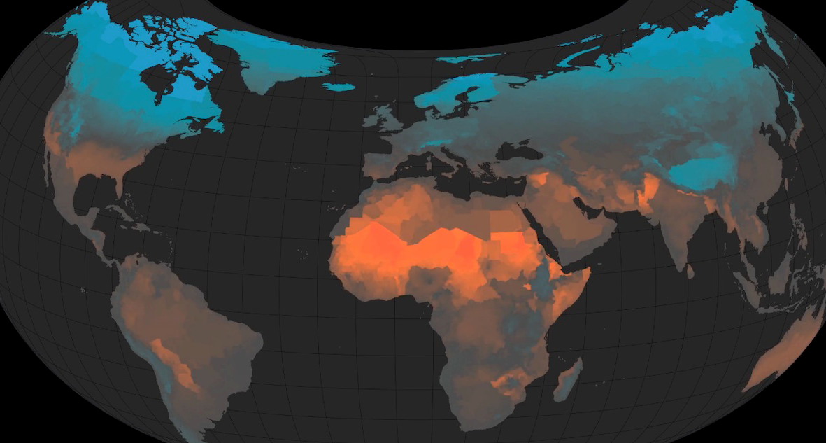
Future emissions depend on a range of factors, including the pace of global economic and population growth, the pace of technological development, and policy decisions. It’s hard to predict these factors over the course of a decade—let alone a century or more—but we know that reducing GHG emissions leads to less warming. Our central scenario in the Lives Saved Calculator is a medium to high emissions pathway, RCP 7.0, that assumes unmitigated emissions growth (O’Neill et al 2016). We map the mean probability outcomes in the globe visualization, and estimate the lives saved and costs avoided using a damage function fitted to the central climate projection. Thus, our point estimates are potentially conservative because they do not evaluate the full range of uncertainty. The incorporation of the full range of uncertainty can increase (or decrease) these estimates due to the convexity of the damage function and how it interacts with temperature trajectories.

Future projections of income and population growth are derived from the Organization for Economic Co-operation and Development (OECD) Env-Growth model (Dellink et al., 2015) and the International Institute for Applied Systems Analysis (IIASA) GDP model (Samir and Lutz, 2014), as part of the “socioeconomic conditions” (population, demographics, education, income, and urbanization projections) of the Shared Socioeconomic Pathways (SSPs). The SSPs propose a set of plausible scenarios of socioeconomic development over the 21^st century in the absence of climate impacts and policy. We emphasize SSP3 because its historic global growth rates in GDP per capita and population match observed global growth rates over the 2000-2018 period much more closely than other SSPs.

To provide useful data about the potential range of outcomes, we also show point estimates of the lives saved and costs avoided for RCP 4.5, a more moderate emissions scenario, and RCP 8.5, a high emissions scenario. The spatially resolved death rates in the map interactive were derived by linearly interpolating RCP 4.5 and RCP 8.5 spatial death rates. In each region and year, the interpolation to RCP 7.0 was weighted by the distance of RCP 7.0 global mean death rates from corresponding global mean death rates under RCP 4.5 and RCP 8.5. Global mean death rates were computed using global mean temperature trajectories for RCP 4.5, RCP 7.0, and RCP 8.5 as simulated by the simple climate model, FaIR, and applying Climate Impact Lab damage functions to those temperatures.

Turning emissions into temperature change

We use the simple climate model, Finite Amplitude Impulse Response (FaIR), to compute the global mean temperature response to the baseline and policy emissions trajectories. FaIR accepts 39 gas emissions species and converts them to atmospheric concentration, radiative forcing, and ultimately temperature change. The model takes into account the carbon cycle and heat exchange between the atmosphere and ocean, including temperature feedbacks on the carbon cycle. State-level emissions of the six greenhouse gases accounted for in our estimates are applied to the FaIR model’s “CO2 fossil”, “CH4”, “N2O”, and “SF6” emissions inputs. State level total hydrofluorocarbons are disaggregated to individual gas emissions species using share of total species in 2012 and input into FaIR, and total perfluorocarbon emissions are applied to FaIR’s “C6F14” emissions input. Units are converted from CO₂ equivalent to native species units expected by FaIR using global warming potentials from the EPA.

There is uncertainty in how sensitive the climate system is to a given change in CO₂ concentration. The climate science community uses a couple metrics to quantify this sensitivity. Equilibrium climate sensitivity (ECS) is how much global mean atmospheric warming occurs due to a doubling of atmospheric CO₂ concentration after the deep ocean has time to respond. This process takes more than 1,000 years. Transient climate response (TCR) is the warming after a gradual increase of CO₂ concentration of 1% per year to its doubling after 70 years. A benefit of using a simple climate model such as FaIR is that it allows for adjustment of the climate sensitivity. For this analysis, we run FaIR with median values of ECS and TCR taken from distributions that represent the full range of climate uncertainty as assessed by the IPCC’s 5^th Assessment Report (AR5) and implemented in the Climate Impact Lab’s work. Global mean temperature evolutions are adjusted to the historical period from 2001 to 2010 to match the base period for our damage functions.

In each year, FaIR converts global emissions to atmospheric concentrations of greenhouse gases using the atmospheric lifetime of each gas. The effect on the energy balance of the climate system (also known as the radiative forcing) is calculated from the changes in concentrations, which leads to a global temperature change. Temperature feeds back onto the carbon cycle such that warming weakens carbon sinks, leading to more CO₂ remaining in the atmosphere.

Turning temperature change into damages

A global mean temperature response consistent with the median climate uncertainty for each of the policy emissions scenarios in each state and the US is converted to deaths and adaptation costs in each year using mean damage functions developed by the Climate Impact Lab. This point estimate of the number of lives saved due to a state’s emissions reduction policy is computed as the difference between the deaths under the baseline “no policy” scenario and the deaths under the “climate mitigation” policy scenario, for each of the given 2050 targets. We report the sum of all lives saved from 2020-2100. The adaptation costs avoided due to a state’s emissions reduction policy is likewise computed as the difference between the costs under the baseline “no policy” scenario and the costs under the given “climate mitigation” policy scenario. We report the sum of all adaptation costs avoided from 2020-2100.

Downscaling state damages to the local level

Lives saved and adaptation costs avoided through 2100 for each state are translated into lives saved and costs avoided for each location—a town, city, or county—by scaling them based on their fractional representation of the state’s population. For example, if Washington state would save 10,000 lives by achieving the target of 100% clean electricity by 2050, and Seattle represents 10% of Washington’s population, then Seattle would save 1,000 lives with a clean electricity policy by this method. This method assumes that emissions scale by population